how to calculate a negative acceleration?

Question

I'm implementing the scrolling behaviour of a touch screen UI but I'm too tired in the moment to wrap my mind around some supposedly trivial piece of math:

y (distance/velocity)
|********
|        ******
|              ****
|                  ***
|                     ***
|                        **
|                          **
|                            *
|                             *
-------------------------------- x (time)

f(x)->?

The UI is supposed to allow the user to drag and "throw" a view in any direction and to keep it scrolling for a while even after he releases the finger from the screen. It's sort of having a momentum that depends on how fast the user was dragging before he took off the finger.

So I have a starting velocity (v0) and every 20ms I scroll by a amount relative to the current velocity. With every scrolling iteration I lower the velocity a bit until it falls below a threshold when I stop it. It just doesn't look right when I decrement it by a fixed amount (linear), so I need to model a negative acceleration but fail to come up with a decent simple formula how to calculate the amount by which I have to lower the velocity in every iteration.

Update:

Thank you for your responses so far but I still didn't manage to derive a satisfying function from the feedback yet. I probably didn't describe the desired solution good enough, so I'll try to give a real world example that should illustrate what kind of calculation I would like to do:

Assume there is a certain car driving on a certain street and the driver hits the brakes to a max until the car comes to a halt. The driver does this with the same car on the same street multiple times but begins to brake at varying velocities. While the car is slowing down I want to be able to calculate the velocity it will have exactly one second later solely based on it's current velocity. For this calculation it should not matter at which speed the car was driving when the driver began to break since all environmential factors remain the same. Of course there will be some constants in the formula but when the car is down to i.e. 30 m/s it will go the same distance in the next second, regardless whether it was driving 100 or 50 m/s when the driver began to break. So the time since hitting the breaks would also not be a parameter of the function. The deceleration at a certain velocity would always be the same.

How do you calculate the velocity one second later in such a situation assuming some arbitrary constants for deceleration, mass, friction or whatever and ignoring complicating influences like air resistance? I'm only after the kinetic energy and the it's dissipation due to the friction from breaking the car.

Update 2 I see now that the acceleration of the car would be liniear and this is actually not what I was looking for. I'll clean this up and try out the new suggestions tomorrow. Thank you for your input so far.

Answer 1

[Short answer (assuming C syntax)]

double v(double old_v, double dt) {
    t = t_for(old_v); 
    new_t = t - dt; 
    return (new_t <= 0)?0:v_for(t);
} 

double t_for(double v) and double v_for(double t) are return values from a v-to-t bidirectional mapping (function in mathematical sence), which is arbitrary with the constraint that it is monothonic and defined for v >=0 (and hence has a point where v=0). An example is:

double v_for(double t) { return pow(t, k); }
double t_for(double v) { return pow(v, 1.0/k); }

where having:

1. k>1 gives deceleration decreasing by modulo as time passes.
2. k<1 gives deceleration increasing by modulo as time passes.
3. k=1 gives constant deceleration.

[A longer one (with rationale and plots)]

So the goal essentialy is:

1. To find a function v(t+dt)=f(v(t),dt) which takes current velocity value v and time delta dt and returns the velocity at the moment t+dt (it does not require actually specifying t since v(t) is already known and supplied as a parameter and dt is just time delta). In other words, the task is to implement a routine double next_v(curr_v, dt); with specific properties (see below).

2. [Please Note] The function in question has a useful (and desired) property of returning the same result regardless of the "history" of previous velocity changes. That means, that, for example, if the series of consecutive velocities is [100, 50, 10, 0] (for the starting velocity v0=100), any other sequence larger than this will have the same "tail": [150, 100, 50, 10, 0] (for the starting velocity v0=150), etc. In other words, regardless of the starting velocity, all velocity-to-time plots will effectively be copies of each other just offset along the time axis each by its own value (see the graph below, note the plots' parts between the lines t=0.0 and t=2.0 are identical) .

3. Besides, acceleration w(t)=dv(t)/dt must be a descending function of time t (for the purpose of visually pleasing and "intuitive" behaviour of the moving GUI object which we model here).

The proposed idea is:

1. First you choose a monothonic velocity function with desired properties (in your case it is gradually decreasing acceleration, though, as the example below shows, it is easier to use "accelerated" ones). This function must not also have an upper boundary, so that you could use it for whatever large velocity values. Also, it must have a point where velocity is zero. Some examples are: v(t) = k*t (not exactly your case, since deceleration k is constant here), v=sqrt(-t) (this one is ok, being defined on the interval t <= 0).

2. Then, for any given velocity, you find the point with this velocity value on the above function's plot (there will be a point, since the function is not bound, and only one since it is monothonic), advance by time delta towards smaller velocity values, thus acquiring the next one. Iteration will gradually (and inevitably) bring you to the point where velocity is zero.

3. That's basically all, there is even no need to produce some "final" formula, dependencies on time value or initial (not current) velocities go away, and the programming becomes really simple.

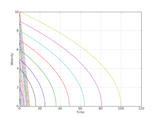
For two simple cases this small python script produces the plots below (initial velocities given were 1.0 to 10.0), and, as you can see, from any given velocity "level" and "downwards" the plots "behave" the same which is of couse because no matter at what velocity you start to slow down (decelerate), you are "moving" along the same curve RELATIVE to the point where velocity is (becomes) zero:

import numpy
import pylab

import math


class VelocityCurve(object):
    """
    An interface for the velocity 'curve'.
    Must represent a _monotonically_ _growing_
        (i.e. with one-to-one correspondence
        between argument and value) function
        (think of a deceleration reverse-played)
    Must be defined for all larger-than-zero 'v' and 't'
    """
    def v(self, t):
        raise NotImplementedError

    def t(self, v):
        raise NotImplementedError



class VelocityValues(object):

    def __init__(self, v0, velocity_curve):
        assert v0 >= 0
        assert velocity_curve

        self._v = v0
        self._vc = velocity_curve

    def next_v(self, dt):
        t = self._vc.t(self._v)
        new_t = t - dt

        if new_t <= 0:
            self._v = 0
        else:
            self._v = self._vc.v(new_t)

        return self._v


class LinearVelocityCurve(VelocityCurve):

    def __init__(self, k):
        """k is for 'v(t)=k*t'"""
        super(LinearVelocityCurve, self).__init__()

        self._k = k

    def v(self, t):
        assert t >= 0
        return self._k*t

    def t(self, v):
        assert v >= 0
        return v/self._k


class RootVelocityCurve(VelocityCurve):

    def __init__(self, k):
        """k is for 'v(t)=t^(1/k)'"""
        super(RootVelocityCurve, self).__init__()

        self._k = k

    def v(self, t):
        assert t >= 0
        return math.pow(t, 1.0/self._k)

    def t(self, v):
        assert v >= 0
        return math.pow(v, self._k)


def plot_v_arr(v0, velocity_curve, dt):
    vel = VelocityValues(v0, velocity_curve)
    v_list = [v0]

    while True:
        v = vel.next_v(dt)
        v_list.append(v)

        if v <= 0:
            break

    v_arr = numpy.array(list(v_list))
    t_arr = numpy.array(xrange(len(v_list)))*dt

    pylab.plot(t_arr, v_arr)


dt = 0.1

for v0 in range(1, 11):
    plot_v_arr(v0, LinearVelocityCurve(1), dt)

for v0 in range(1, 11):
    plot_v_arr(v0, RootVelocityCurve(2), dt)


pylab.xlabel('Time ')
pylab.ylabel('Velocity')

pylab.grid(True)

pylab.show()

This gives the following plots (linear ones for the linear decelerating (i.e. constant deceleration), "curvy" -- for the case of the "square root" one (see the code above)):

Also please beware that to run the above script one needs pylab, numpy and friends installed (but only for the plotting part, the "core" classes depend on nothing and can be of course used on their own).

P.S. With this approach, one can really "construct" (for example, augmenting different functions for different t intervals or even smoothing a hand-drawn (recorded) "ergonomic" curve) a "drag" he likes:)

Answer 2

After reading the comments, I'd like to change my answer: Multiply the velocity by k < 1, like k = 0.955, to make it decay exponentially.

Explanation (with graphs, and a tuneable equation!) follows...

I interpret the graph in your original question as showing velocity staying near the starting value, then decreasing increasingly rapidly. But if you imagine sliding a book across a table, it moves away from you quickly, then slows down, then coasts to a stop. I agree with @Chris Farmer that the right model to use is a drag force that is proportional to speed. I'm going to take this model and derive the answer I suggested above. I apologize in advance for the length of this. I'm sure someone better at math could simplify this considerably. Also, I put links to the graphs in directly, there are some characters in the links that the SO parser doesn't like. URLs fixed now.

I'm going to use the following definitions:

x -> time
a(x) -> acceleration as a function of time
v(x) -> velocity as a function of time
y(x) -> position as a function of time
u -> constant coefficient of drag
colon : denotes proportionality

We know that the force due to drag is proportional to speed. We also know that force is proportional to acceleration.

a(x) : -u v(x)        (Eqn. 1)

The minus sign ensures that the acceleration is opposite the current direction of travel.

We know that velocity is the integrated acceleration.

v(x) : integral( -u v(x) dx )        (Eqn. 2)

This means the velocity is proportional to its own integral. We know that e^x satisfies this condition. So we suppose that

v(x) : e^(-u x)        (Eqn. 3)

The drag coefficient in the exponent is so that when we solve the integral in Eqn. 2 the u cancels to get back to Eqn. 3.

Now we need to figure out the value of u. As @BlueRaja pointed out, e^x never equals zero, regardless of x. But it approaches zero for sufficiently negative x. Let's consider 1% of our original speed to be 'stopped' (your idea of a threshold), and let's say we want to stop within x = 2 seconds (you can tune this later). Then we need to solve

e^(-2u) = 0.01        (Eqn. 4)

which leads us to calculate

u = -ln(0.01)/2 ~= 2.3        (Eqn. 5)

Let's graph v(x).

Looks like it exponentially decays to a small value in 2 seconds. So far, so good.

We don't necessarily want to calculate exponentials in our GUI. We know that we can convert exponential bases easily,

e^(-u x) = (e^-u)^x        (Eqn. 6)

We also don't want to keep track of time in seconds. We know we have an update rate of 20 ms, so let's define a timetick n with a tick rate of 50 ticks/sec.

n = 50 x        (Eqn. 7)

Substituting the value of u from Eqn. 5 into Eqn. 6, combining with Eqn. 7, and substituting into Eqn. 3, we get

v(n) : k^n, k = e^(ln(0.01)/2/50) ~= 0.955        (Eqn. 8)

Let's plot this with our new x-axis in timeticks.

Again, our velocity function is proportional to something that decays to 1% in the desired number of iterations, and follows a 'coasting under the influence of friction' model. We can now multiply our initial velocity v0 by Eqn. 8 to get the actual velocity at any timestep n:

v(n) = v0 k^n        (Eqn. 9)

Note that in implementation, it is not necessary to keep track of v0! We can convert the closed form v0 * k^n to a recursion to get the final answer

v(n+1) = v(n)*k        (Eqn. 10)

This answer satisfies your constraint of not caring what the initial velocity is - the next velocity can always be calculated using just the current velocity.

It's worth checking to make sure the position behavior makes sense. The position following such a velocity model is

y(n) = y0 + sum(0..n)(v(n))        (Eqn. 11)

The sum in Eqn. 11 is easily solved using the form of Eqn 9. Using an index variable p:

sum(p = 0..n-1)(v0 k^p) = v0 (1-k^n)/(1-k)        (Eqn. 12)

So we have

y(n) = y0 + v0 (1-k^n)/(1-k)        (Eqn. 13)

Let's plot this with y0 = 0 and v0 = 1.

So we see a rapid move away from the origin, followed a graceful coast to a stop. I believe this graph is a more faithful depiction of sliding than your original graph.

In general, you can tune k by using the equation

k = e^(ln(Threshold)/Time/Tickrate)        (Eqn. 14)
where:
Threshold is the fraction of starting velocity at which static friction kicks in
Time is the time in seconds at which the speed should drop to Threshold
Tickrate is your discrete sampling interval

(THANKS to @poke for demonstrating the use of Wolfram Alpha for plots - that's pretty sweet.)

OLD ANSWER

Multiply the velocity by k < 1, like k = 0.98, to make it decay exponentially.